Improved visualization of discontinuous fields
The visualization of the results obtained from MagnetoDynamicsCalcFields, and other discontinuous fields, have been somewhat suboptimal until recently. Particularly with the adoption of quadratic edge elements the old options were no longer satisfactory. This mail summarizes the recent changes related to the optimal visualization. I hope that with these new features the excellent 2nd order edge elements can show their full potential, but also the 1st order edge elements will benefit from these. The text is related to the current devel version.
The CalcFields solver can basically compute nodal quantities and elemental quantities. For fields known to be continuous the nodal quantities are good as such. However, for quantities having potential jumps between element interfaces (such as current density) the elemental fields are much more suitable. The elemental fields are actually standard nodal fields with the degrees of freedom being independent in each element (as in the Discontinuous Galerkin method). This makes the amount of data potentially quite huge. One may choose between three different ways to save the results in VTU output:
- Constant (averaged Cell data) within each element (default)
- “Discontinuous Galerkin” data where all nodes are different in each elements
- “Discontinuous Bodies” data where nodes are made different only at the interfaces.
The preferred method of choice for visualization is usually the 3rd one. It also automatically averages the different shared instances of the DG fields to one single value. Unfortunately for quadratic elements there seems to be a problem. It seems that the rendering in Paraview cannot handle discontinuities well in conjunction with quadratic elements. To overcome that problem there is a possibility to save the result in linear basis even though having quadratic mesh. Actually this may make sense since the derived fields are still often just linear in accuracy.
Below is an example of a sif file that seems to provide nice visualizations for a number of cases both in serial and parallel
Solver 3
  Exec Solver = after timestep
  Equation = "ResultOutput"
  Procedure = "ResultOutputSolve" "ResultOutputSolver"
  Output File Name = f
  Vtu format = True
  Discontinuous Bodies = True
  ! bloated alternative for the above maintaining all discontinuities
  ! Discontinuous Galerkin = True
  Save Geometry Ids = True
  ! use this only in conjunction with quadratic mesh
  Save Linear Elements = True
  ! Save Bulk Only = True
  ! Save Boundaries Only = True
End
Unfortunately there is some loss of information when performing these
operations and line plotting in Paraview is not optimal. The alternative
is to save the data directly using SaveLine. Previously this routine had
problems with discontinuous fields also since it only saves data at the
intersection of faces, and assumes value in between to be linear. If the
face values are not unique this does not work. Now there is a remedy to
give number of divisions for each line. When using the “Polyline
Divisions” to specify the points also the DG fields are considered
correctly, for example
Solver 4
  Exec Solver = after timestep
  Equation = SaveLine
  Procedure = "SaveData" "SaveLine"
  Filename = g.dat
  Polyline Coordinates(8,3) =  0   -0.05  -0.07  0    -0.05 0.115  \
                               0.0  0.05  -0.07  0.0   0.05 0.115 \
                              -0.05 0.0   -0.07 -0.05  0.0  0.115 \
                               0.05 0.0   -0.07  0.05  0.0  0.115
  Polyline Divisions(4) = 100 100 100 100
End
Note that if one chooses “Discontinuous Bodies” in the VTU output it
averages the data. Hence if you want the original discontinuous (linear or
quadratic) data give this solver a smaller Id number than for the
ResultOutputSolver.
Finally there is a possibility to also use SaveGridData solver would you
want to save the data in a uniform grid. This also now works with DG
fields and can therefore capture the true results from CalcFields. This is
probably not that useful, but an example is provided here for
completeness.
Solver 5
  Equation = SaveGridData
  Procedure = "SaveGridData" "SaveGridData"
  Grid dx = Real 0.05
  Grid dy = Real 0.05
  Grid dz = Real 0.00005

! Reduce the box where the points are saved in
  Min Coordinate 1 = Real -0.07
  Max Coordinate 1 = Real 0.07
  Min Coordinate 2 = Real -0.07
  Max Coordinate 2 = Real 0.07

! If nodes are exactly at the interface eliminate redundant ones
  Check For Duplicates = Logical True
  Binary Output = Logical True
  Single Precision = Logical True

  Filename Prefix = h

! save in vtu format in paraview (use glyphs)
  Vtu Format = Logical True

! save in ascii format for Matlab etc.
  Table Format = Logical True
End
I hope people using the great MagnetodDynamics solver will find these instructions useful.